With the election days away, it is time to make my final prediction for the 2024 US Presidential Election. In the past weeks, I have alternated between Electoral College predictions and National Popular Vote predictions. For the final prediction blog post, I will predict both of these using the methods and data I have explored in previous posts.
National Prediction
The first prediction I will explore is the National Prediction. This prediction will predict the Two-Party Vote Share for both Kamala Harris and Donald Trump
Fundamental Model Description, Justification, and Formula
The final model is an ensemble of two models. Due to the large impact that the data from the 2020 election has on prediction models. I made two models, one with the 2020 data and one without it.
The first model is a “fundamental” model using a simple OLS regression. The first model utilizes economic data from the Federal Reserve FRED database. The economic inputs to the model are from the second quarter of election years. The inputs are GDP quarterly growth, Consumer Price Index (inflation), homeowner vacancy, rental vacancy, and volatility of the stock market (difference between high and low in the quarter). GDP quarterly growth and the volatility of the stock market are incldued in the model to get a general sense of the state of the economy. The rest of the economic variables are inlcuded due to their relevance in the 2024 election. Homeowner vacancy and rnetal vacancy are designed to capture the effects that the housing crisis will have on the election. Despite recent improvement, inflation is included in the model as it remains important to voters.
Below is the summary statistics for the two regression. The left column represents the model with 2020 data included. The right side is without 2020 included. The statistics show that the right side model’s GDP growth is more significant than the left. Additionally, the R^2 on the right side model is higher suggesting that it better explains the variance in the data. Notably though most coefficents are not significant.
##
## ==========================================================
##                               Dependent variable:
##                      -------------------------------------
##                                      pv2p
##                             (1)                (2)
## ----------------------------------------------------------
## GDP_growth_quarterly       0.484*            0.713**
##                           (0.248)            (0.303)
##
## sp500move                  0.036              -0.018
##                           (0.037)            (0.056)
##
## CPI                        -0.029             -0.014
##                           (0.035)            (0.037)
##
## homeowner_vacancy          -1.161             0.551
##                           (4.902)            (4.965)
##
## rental_vacancy             -0.371             -0.304
##                           (1.162)            (1.133)
##
## Constant                 57.457***          53.566***
##                           (6.407)            (6.963)
##
## ----------------------------------------------------------
## Observations                 17                 16
## R2                         0.390              0.447
## Adjusted R2                0.112              0.170
## Residual Std. Error   4.921 (df = 11)    4.794 (df = 10)
## F Statistic          1.405 (df = 5; 11) 1.616 (df = 5; 10)
## ==========================================================
## Note:                          *p<0.1; **p<0.05; ***p<0.01
While the right side model performs better in-sample, the left side model performs better out of sample. Calculating mean error after running 1000 simulations of cross-validation, the left side all data model had mean error of 6.65 while the right side model had a mean error of 9.98.
Polling Model Description, Justification, and Formula
The second model for the ensemble is based off polling data. The polling data used within the model is the averages from 538. Similar to the fundamental model, I also created two polling models. The first inlcudes all data and the second removes the 2020 and 2016 elections due to perceived polling misses. The two models where created using elastic-net to create a model that considers each polling average from 30 weeks out from the election until now.
The model with all data included performed better out of sample as it had a mean squared error of 57.1 compared to the second model’s mean squared error of 91.4.
In both the fundamental and polling models, the prediction intervals were extremely wide and crossed over the 50% vote threshold
Ensembling and Final Prediction
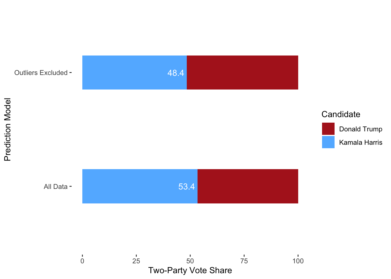
Below are the final prediction for the two models. In both models, the fundamental model is weighted to be 2/3 of the prediction compared to 1/3 of the prediction for the polling model. This decision was made to the higher R^2 for the fundamental model and the perceived inaccuracy of polling in recent years.
Overall, I believe more in the all data model because elections happen so rarely that more data is better. Additionally, the all data model for both the fundamental and polling models performed better out of sample.

State Prediction
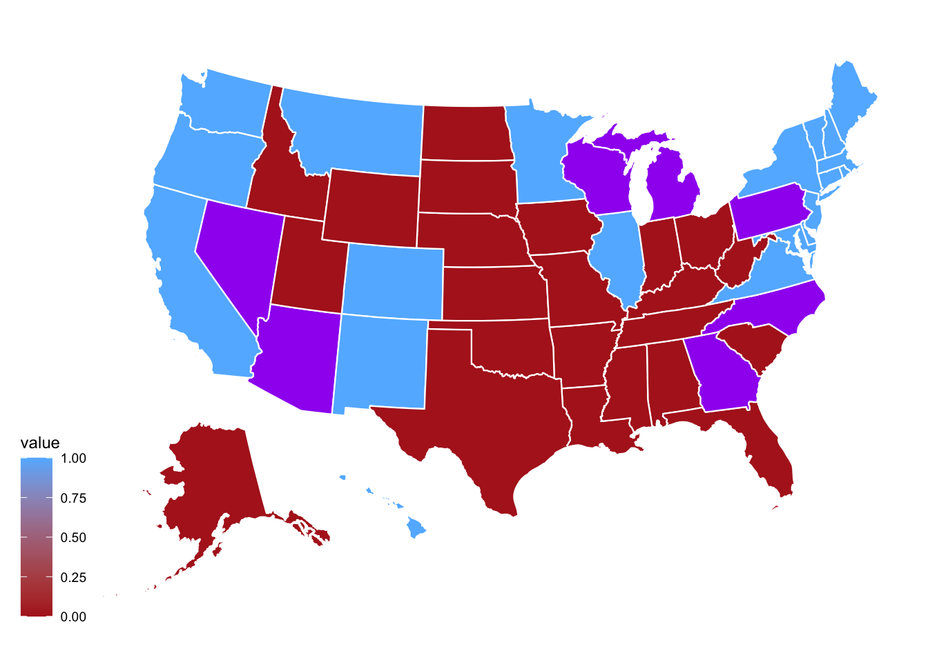
For the state prediction, I decided to only create models for the state that were tossusps. To determine which states were tossups, I used the race ratings from Cook Politcal Report. The seven tossup states are highlighted below in purple on the map

Model Description, Justification, and Formula
Similar to the national model, the state prediction models combine polling data and fundamental economic data. The model uses historical polling in each state to predict based on the 2024 polling averages. The model also uses national GDP quarter two growth and inflation (CPI). For the final prediction the model weighs polling data 2/3 and fundamental economic data 1/3 due to polling data being more in tune with interesting shocks in 2024. If I were using state level economic data, I would consider giving it a higher weight.
In Sample Results of the Fundamental State Models
Below are the in-sample results of the fundamental state models. The columns are in alphabetical order from Arizona to Wisconsin. In all of the models, the economic variables are very significant. However, the R^2 is on the lower side in most states except North Carolina.
##
## ==================================================================================================
##                                                   Dependent variable:
##                      -----------------------------------------------------------------------------
##                                                         D_pv2p
##                                 (1)                       (2)                       (3)
## --------------------------------------------------------------------------------------------------
## GDP_growth_quarterly         -0.020**                  -0.199***                 0.167***
##                               (0.008)                   (0.007)                   (0.008)
##
## CPI                          0.033***                  -0.041***                 0.043***
##                               (0.002)                   (0.002)                   (0.001)
##
## Constant                     40.107***                 55.747***                 44.698***
##                               (0.351)                   (0.329)                   (0.252)
##
## --------------------------------------------------------------------------------------------------
## Observations                   2,198                     1,891                     2,376
## R2                             0.217                     0.330                     0.314
## Adjusted R2                    0.217                     0.329                     0.314
## Residual Std. Error      3.194 (df = 2195)         2.746 (df = 1888)         3.298 (df = 2373)
## F Statistic          304.909*** (df = 2; 2195) 464.810*** (df = 2; 1888) 543.841*** (df = 2; 2373)
## ==================================================================================================
## Note:                                                                  *p<0.1; **p<0.05; ***p<0.01
##
## ====================================================================================================
##                                                    Dependent variable:
##                      -------------------------------------------------------------------------------
##                                                          D_pv2p
##                                  (1)                        (2)                       (3)
## ----------------------------------------------------------------------------------------------------
## GDP_growth_quarterly          0.205***                   -0.040***                 0.100***
##                                (0.007)                    (0.008)                   (0.006)
##
## CPI                           0.115***                   0.039***                  0.010***
##                                (0.002)                    (0.002)                   (0.001)
##
## Constant                      27.120***                  39.348***                 50.469***
##                                (0.336)                    (0.295)                   (0.283)
##
## ----------------------------------------------------------------------------------------------------
## Observations                    1,874                      2,307                     2,114
## R2                              0.720                      0.326                     0.107
## Adjusted R2                     0.719                      0.326                     0.107
## Residual Std. Error       2.780 (df = 1871)          3.394 (df = 2304)         2.567 (df = 2111)
## F Statistic          2,403.034*** (df = 2; 1871) 557.566*** (df = 2; 2304) 127.019*** (df = 2; 2111)
## ====================================================================================================
## Note:                                                                    *p<0.1; **p<0.05; ***p<0.01
##
## ================================================
##                          Dependent variable:
##                      ---------------------------
##                                D_pv2p
## ------------------------------------------------
## GDP_growth_quarterly          0.111***
##                                (0.007)
##
## CPI                           0.016***
##                                (0.001)
##
## Constant                      49.211***
##                                (0.272)
##
## ------------------------------------------------
## Observations                    2,211
## R2                              0.116
## Adjusted R2                     0.115
## Residual Std. Error       2.692 (df = 2208)
## F Statistic           145.037*** (df = 2; 2208)
## ================================================
## Note:                *p<0.1; **p<0.05; ***p<0.01
Out of Sample Results of the Fundamental State Models
| State | Out of Sample Error |
|---|---|
| Arizona | 4.49 |
| Georgia | 3.74 |
| Michigan | 2.92 |
| Nevada | 3.91 |
| North Carolina | 4.16 |
| Pennsylvania | 2.91 |
| Wisconsin | 2.76 |
In Sample Results of the Polling State Models
Below are the in-sample results of the polling state models. The columns are in alphabetical order from Arizona to Wisconsin. In all of the models, the poll support is very significant. However, the R^2 is extremely low in most states except Nevada.
##
## ================================================================================================
##                                                 Dependent variable:
##                     ----------------------------------------------------------------------------
##                                                        D_pv2p
##                               (1)                       (2)                       (3)
## ------------------------------------------------------------------------------------------------
## poll_support                0.093***                 0.315***                  0.228***
##                             (0.012)                   (0.017)                   (0.013)
##
## Constant                   42.809***                 34.742***                 42.609***
##                             (0.485)                   (0.723)                   (0.579)
##
## ------------------------------------------------------------------------------------------------
## Observations                 2,189                     1,883                     2,369
## R2                           0.026                     0.147                     0.113
## Adjusted R2                  0.025                     0.147                     0.113
## Residual Std. Error    3.533 (df = 2187)         2.914 (df = 1881)         3.730 (df = 2367)
## F Statistic         57.253*** (df = 1; 2187) 325.050*** (df = 1; 1881) 302.945*** (df = 1; 2367)
## ================================================================================================
## Note:                                                                *p<0.1; **p<0.05; ***p<0.01
##
## ==================================================================================================
##                                                  Dependent variable:
##                     ------------------------------------------------------------------------------
##                                                         D_pv2p
##                                 (1)                        (2)                      (3)
## --------------------------------------------------------------------------------------------------
## poll_support                 0.730***                   0.340***                 -0.059***
##                               (0.019)                    (0.014)                  (0.012)
##
## Constant                     18.334***                  32.213***                54.992***
##                               (0.820)                    (0.609)                  (0.518)
##
## --------------------------------------------------------------------------------------------------
## Observations                   1,865                      2,301                    2,107
## R2                             0.445                      0.197                    0.012
## Adjusted R2                    0.444                      0.197                    0.012
## Residual Std. Error      3.893 (df = 1863)          3.685 (df = 2299)        2.679 (df = 2105)
## F Statistic         1,492.239*** (df = 1; 1863) 564.187*** (df = 1; 2299) 26.135*** (df = 1; 2105)
## ==================================================================================================
## Note:                                                                  *p<0.1; **p<0.05; ***p<0.01
##
## ===============================================
##                         Dependent variable:
##                     ---------------------------
##                               D_pv2p
## -----------------------------------------------
## poll_support                 0.169***
##                               (0.009)
##
## Constant                     44.516***
##                               (0.407)
##
## -----------------------------------------------
## Observations                   2,203
## R2                             0.141
## Adjusted R2                    0.140
## Residual Std. Error      2.617 (df = 2201)
## F Statistic          360.473*** (df = 1; 2201)
## ===============================================
## Note:               *p<0.1; **p<0.05; ***p<0.01
Out of Sample Results of the Polling State Models
| State | Out of Sample Error |
|---|---|
| Arizona | 2.49 |
| Georgia | 2.26 |
| Michigan | 2.29 |
| Nevada | 2.78 |
| North Carolina | 1.88 |
| Pennsylvania | 1.91 |
| Wisconsin | 1.73 |
Below are the prediction intervals of the state models. North Carolina and Arizona stand out as their prediction intervals cross the 50% vote threshold. Additionally, North Carolina has the largest interval out of all the state models.

Final Electoral College Prediction
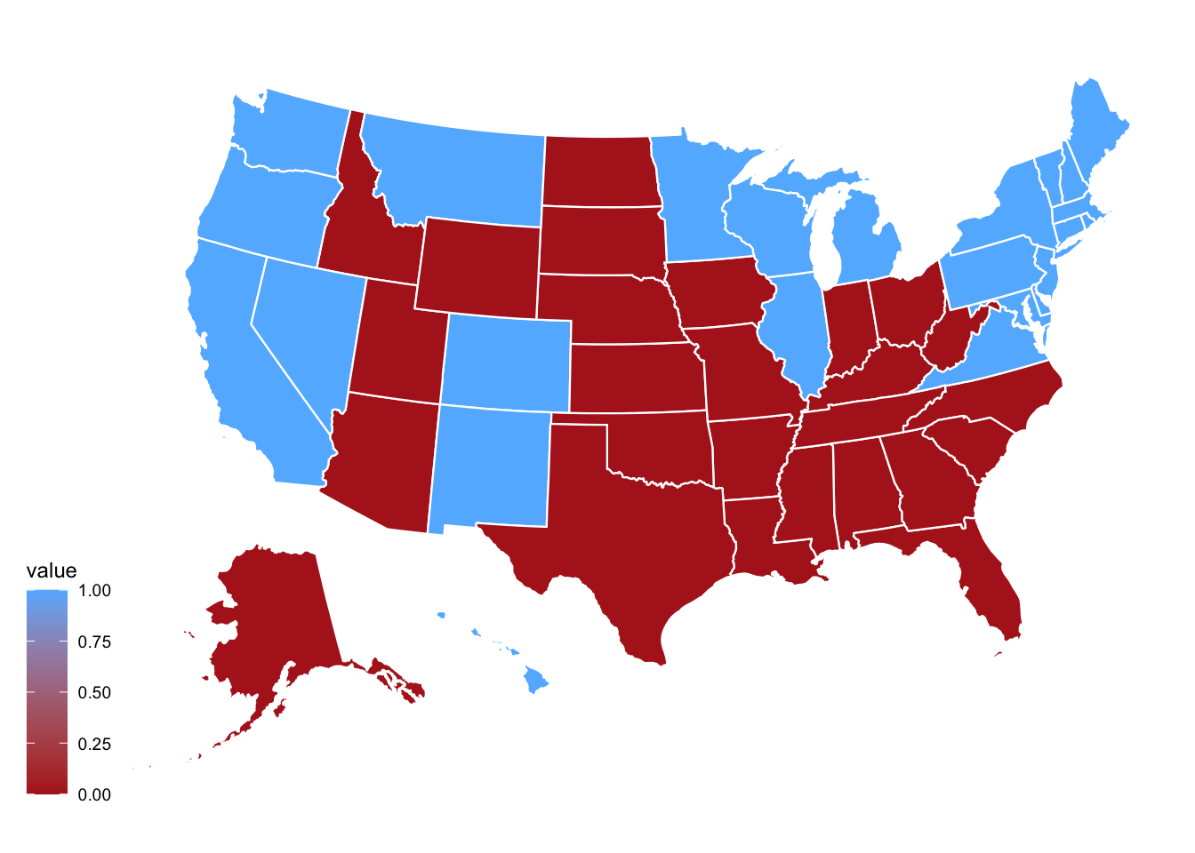
The individual state models predict a close election with Kamala Harris winning Michigan, Wisconsin, Pennsylvania and Trump winning Arizona, Georgia, North Carolina. This would result in Harris winning the Electoral College with exactly 270 votes.

Listed below are the predicted two-party vote shares from the state models.
| State | Harris Predicted Two-Party Vote | Trump Predicted Two-Party Vote |
|---|---|---|
| Arizona | 48.0% | 52.0% |
| Georgia | 46.5% | 53.5% |
| Michigan | 54.6% | 45.4% |
| Nevada | 54.2% | 45.8% |
| North Carolina | 48.6% | 51.4% |
| Pennsylvania | 52.9% | 47.1% |
| Wisconsin | 52.7% | 47.3% |